Overview

Teaching: 20 min
Exercises: 10 min

Questions

• How can you keep data clean and sane?

Objectives

• Apply quality assurance techniques to limit incorrect data entry.

• Apply quality control techniques to identify errors in spreadsheets.

• Get to know filtering and its benefits.

When you have a well-structured data table, you can use several simple techniques within your spreadsheet to ensure the data you enter is free of errors. These approaches include techniques that are implemented prior to entering data (quality assurance) and techniques that are used after entering data to check for errors (quality control).

Quality Assurance

Quality assurance stops bad data from ever being entered by checking to see if values are valid during data entry. For example, if research is being conducted at sites A, B, and C, then the value V (which is right next to B on the keyboard) should never be entered. Likewise if one of the kinds of data being collected is a count, only integers greater than or equal to zero should be allowed.

To control the kind of data entered into a a spreadsheet we use Data Validation (Excel) or Validity (LibreOffice Calc), to set the values that can be entered in each data column.

1. Select the cells or column you want to validate

2. On the Data tab select Data Validation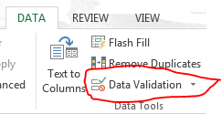

   

3. In the Allow box select the kind of data that should be in the column. Options include whole numbers, decimals, lists of items, dates, and other values.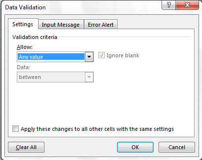

   

4. After selecting an item enter any additional details. For example if you’ve chosen a list of values then enter a comma-delimited list of allowable values in the Source box.

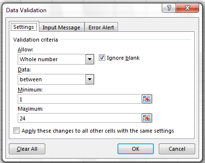
We can’t have half a person attending a workshop, so let’s try this out by setting the num_registered column in our spreadsheet to only allow whole numbers between 1 and 100.

1. Select the num_registered column
2. On the Data tab select Data Validation
3. In the Allow box select Whole number
4. Set the minimum and maximum values to 1 and 100.

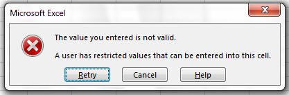
Now let’s try entering a new value in the plot column that isn’t a valid plot. The spreadsheet stops us from entering the wrong value and asks us if we would like to try again.

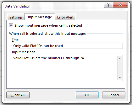
You can also customize the resulting message to be more informative by entering your own message in the Input Message tab

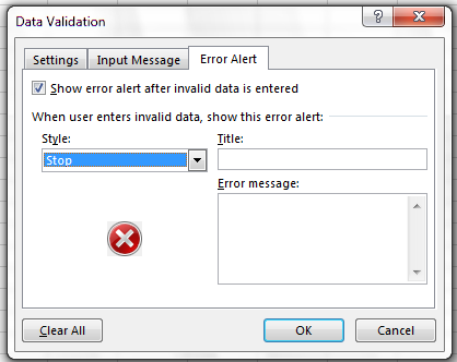
and allow invalid data to just result in a warning by modifying the Style option on the Error Alert tab.

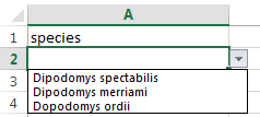
Quality assurance can make data entry easier as well as more robust. For example, if you use a list of options to restrict data entry, the spreadsheet will provide you with a drop-downlist of the available items. So, instead of trying to remember the initials of all your trainers, you can just select the right option from the list.

Quality Control

Tip!

Before doing any quality control operations, save your original file with the formulas and a name indicating it is the original data. Create a separate file with appropriate naming and versioning, and ensure your data is stored as values and not as formulas. Because formulas refer to other cells, and you may be moving cells around, you may compromise the integrity of your data if you do not take this step!

readMe (README) files: As you start manipulating your data files, create a readMe document / text file to keep track of your files and document your manipulations so that they may be easily understood and replicated, either by your future self or by an independent researcher. Your readMe file should document all of the files in your data set (including documentation), describe their content and format, and lay out the organizing principles of folders and subfolders. For each of the separate files listed, it is a good idea to document the manipulations or analyses that were carried out on those data.

Sorting

Bad values often sort to bottom or top of the column. For example, if your data should be numeric, then alphabetical and null data will group at the ends of the sorted data. Sort your data by each field, one at a time. Scan through each column, but pay the most attention to the top and the bottom of a column. If your dataset is well-structured and does not contain formulas, sorting should never affect the integrity of your dataset.

Exercise

Open a new spreadsheet on Excel and in the column A type in 4, 2h, 3h, 5, 4, 6, 1, downward for each cell in that order. Go to the ‘Data’ tab and switch between sorting ascending and descending by clicking AZ↓ and the AZ↑

You see how no matter the sorting, the incorrectly entered values 2h, 3h, always end up at the bottom or top of the column. This way you can check for values that do not follow the expected trend beacuse of improper entry.

Conditional formatting

Use with caution! But a great way to flag inconsistent values when entering data.

Conditional formatting basically can do something like color code your values by some criteria or lowest to highest. This makes it easy to scan your data for outliers.

Exercise

In Excel, select the same column in the previous example and delete the 2h and 3h entries and go to the ‘Home’ tab.
Here you will find the button Conditional formatting. Play around with it by holding the mouse cursor above different ‘Data bars’, ‘Color scales’ and ‘Icon sets’ without clicking. You can also try some of the ‘Highlight Cells Rules’ and ‘Top/Bottom’ rules.

Note that conditional formatting only works with numbers and not text.

PS. This coloration can be very confusing to people who do not know about conditional formatting, so make sure that if you use this functionality, comment this somewhere fitting.

PPS. To remove the formatting, select the cell or the column, click on ‘Conditional formatting’, go down to ‘Clear rules’ -> Clear rules from selected cells’.

Filtering as an alternative to restructuring data

Sometimes, rather than tidying your data by deleting rows, copying rows or making additional tables from your data, it can be more versatile to use the Filter functionalities of your spreadsheet program. Filtering, in addition to sorting your data, allows you to hide or show data of your choosing, for example only cells with a certain collection value.

Let’s do some exercises to show what you can do with tihe filtering functionality in Excel.

Exercise

Open the ‘Lending 30 days_overdue.xlsx’ file with the unmerged ‘Due Date’ column. If you don’t have it, you can download it with the unmerged column here: Lending_30 days_overdue_unmerged.xlsx. Select the header row (the one with ‘External Request Id’) and click on the Filter button in the ‘Data’ tab.
You should see that the header row now has a little triangle in each cell. By clicking on these triangles you get access to the functionalities of the Excel filtering. You are probably already quite familiar with sorting by now, so let’s try filtering on values.

1. Click on the header ‘Lending Request Status’ and uncheck Select all and check the values you want to display.
   Play around and try out filtering multiple columns on the values you want.
   (To remove filter, click ‘Clear filter from …’ in the Filter menu).
2. Note that you have quite detailed filtering options on ‘Due Date’ (click the little plus sign).
3. Try sorting the filtered columns.
4. Try selecting a fitlered result and copy the contents into a new sheet. What happened to the content?

Key Points

• Use data validation tools to minimise the possibility of input errors.

• Use sorting and conditional formatting to identify possibly errors.

• Use filtering as an alternative to tidying of data.