A short introduction to machine learning#
Machine learning is really just fancy statistics. Still, machine learning is fun, and here we’ll take a look at what we can do. There are three major types of machine learning:
Supervised learning
Unsupervised learning
Reinforcement learning
Here, we will only discuss supervised and unsupervised learning.
But first, we will need to import some libraries for machine learning.
scikit-learn (
sklearn) is a toolkit for machine learningmatplotlib is a library for plotting and visualizing results
numpy is a package for scientific computing with Python
import matplotlib.pyplot as plt
from matplotlib.colors import ListedColormap
from sklearn.model_selection import train_test_split
from sklearn.datasets import make_moons, make_circles, make_classification, make_blobs
from sklearn.neighbors import KNeighborsClassifier
from sklearn.svm import SVC
from sklearn.cluster import KMeans
from sklearn.linear_model import Perceptron
from sklearn.neural_network import MLPClassifier
import numpy as np

# define colors
colors = plt.cm.RdBu
colors_bright = ListedColormap(['#FF0000', '#0000FF'])
Supervised learning: classification#
By supervision we mean human supervision. Supervised learning works with labeled (annotated) data. The labels must be made manually by people, and this can require a lot of work for large data sets.
A common machine learning task is classification of items. That is, determining which group or class an item belongs to. Neural networks are powerful classifiers that can be used with complex data sets. But there are also many simpler classifiers. We will try a couple of different non-neural classifiers, and then try neural networks in an exercise.
Before we start coding the machine learning part, we will need a way to visualize the results. Below, we define a function to plot the decision boundary produced by classifier. The details of this function are not important, so you don’t need to spend much time understanding it.
def plot_boundary(classifier, data, datasets):
    X_train, X_test, y_train, y_test = datasets
    score = classifier.score(X_test, y_test)
    figure = plt.figure(figsize=(7, 7))
    h = .02  # step size in the mesh
    x_min, x_max = data[:, 0].min() - .5, data[:, 0].max() + .5
    y_min, y_max = data[:, 1].min() - .5, data[:, 1].max() + .5
    xx, yy = np.meshgrid(np.arange(x_min, x_max, h),
                         np.arange(y_min, y_max, h))

    # Plot the decision boundary. For that, we will assign a color to each
    # point in the mesh [x_min, x_max]x[y_min, y_max].
    if hasattr(classifier, "decision_function"):
        Z = classifier.decision_function(np.c_[xx.ravel(), yy.ravel()])
    else:
        Z = classifier.predict_proba(np.c_[xx.ravel(), yy.ravel()])[:, 1]

    # Put the result into a color plot
    Z = Z.reshape(xx.shape)
    plt.contourf(xx, yy, Z, cmap=colors, alpha=.8)

    # Plot the training points
    plt.scatter(X_train[:, 0], X_train[:, 1], c=y_train, cmap=colors_bright,
               edgecolors='k')
    # Plot the testing points
    plt.scatter(X_test[:, 0], X_test[:, 1], c=y_test, cmap=colors_bright,
               edgecolors='k', alpha=0.6)

    #add labels
    plt.xlabel('lazy - active')
    plt.ylabel('size')
    plt.text(xx.max() - .3, yy.min() + .3, ('%.2f' % score),
             size=15, horizontalalignment='right')
    plt.show()
Next, we need some data to work with. As an example, we will use a simulated, random data set.
data, labels = make_classification(n_features=2, n_redundant=0, n_informative=2,
                                   random_state=2, n_clusters_per_class=1)
We can examine the data:
print(data)
[[-0.53217655  0.62924614]
 [ 0.91255258  1.83216496]
 [-1.01552104  1.32130405]
 [-1.72720358  2.01580762]
 [ 0.57936765 -0.17841637]
 [-1.96704317  2.7884374 ]
 [ 1.58793772 -0.50958635]
 [-0.65431412  5.42498149]
 [-0.15506497  4.71531042]
 [-0.32922076 -0.38114073]
 [-0.82129175 -0.42577634]
 [ 0.81367196  1.55193973]
 [-0.56552887  0.86413142]
 [-0.11874769  2.41406082]
 [-1.01918239  0.9304136 ]
 [ 0.86896538  0.43455506]
 [ 1.56022402 -0.5928549 ]
 [ 2.51074961  2.20851363]
 [-0.68589017  0.45250806]
 [-0.6395146   0.22675732]
 [-0.14861319  0.20800257]
 [ 0.79669069  0.6008606 ]
 [-0.9159984   1.46858828]
 [ 0.86716721 -0.21053434]
 [ 1.20449563 -0.50069527]
 [ 0.48099044  2.45911181]
 [ 0.72536994  0.14125124]
 [-0.230009   -0.88509835]
 [-1.21074582  1.98824465]
 [ 1.90443572  1.09668944]
 [-0.49740529  0.55464122]
 [-1.2242189   0.3946374 ]
 [ 1.80228789  0.1624976 ]
 [-0.12641848 -0.22493973]
 [-0.98006945  0.27323875]
 [ 0.02996952 -0.42072336]
 [-0.50289181 -0.47970246]
 [-1.50713655  1.88231496]
 [ 1.74522591  0.26945127]
 [ 1.22087596  1.80015056]
 [-0.13481863  2.47359132]
 [-1.10470103  1.31877761]
 [ 1.13845568  1.5207657 ]
 [-0.25009045 -0.99239407]
 [-1.02761317  0.82744651]
 [ 0.09698618  1.14574985]
 [-0.83929907  0.57095256]
 [ 1.25687802  2.50091971]
 [ 0.28879378  1.91506166]
 [ 0.90992454  2.16315303]
 [ 1.14781769 -0.21008363]
 [ 1.19867229  1.49447345]
 [ 0.87102184  0.36242782]
 [ 1.36034198 -0.35367049]
 [-0.7462074   0.94164777]
 [-0.47005586  0.43835818]
 [-0.60735425  1.18433877]
 [-1.01138792  0.58059624]
 [-1.20224699  1.7468454 ]
 [ 0.63369838  1.19841252]
 [-0.87235494  0.82088891]
 [-0.4888825   1.04134073]
 [-1.42154875  1.21208496]
 [-0.81927204  1.3192171 ]
 [ 2.19637546  0.06666848]
 [ 0.69665507  1.58016304]
 [ 0.69222025 -1.69526178]
 [-1.25936374  1.59043789]
 [-0.76909262  0.39791467]
 [-1.07205058  0.92274897]
 [ 0.9103046   2.36350736]
 [ 1.38658288  0.9350742 ]
 [-0.54679798  0.42400179]
 [-0.88737112 -0.45412572]
 [-0.86879403 -0.17160316]
 [-0.80332327  0.94271177]
 [-0.92016356  0.49074041]
 [-1.51031122  1.43848761]
 [ 1.33356724  1.55909192]
 [-1.29098079  0.84130386]
 [-1.06725963  2.59573622]
 [-1.3947416   1.62017245]
 [ 2.12934709  0.33816429]
 [-1.51622684  1.31067916]
 [-1.4324849   1.56116588]
 [-1.82111157  2.36975108]
 [-0.79130409  0.73911266]
 [ 1.05891574 -0.02984642]
 [ 1.50039251  0.86208641]
 [-0.95495832  0.5743687 ]
 [ 0.3031273   1.80172827]
 [ 1.1442031   1.70630765]
 [-0.95320937  0.75310075]
 [-1.00777547  0.82420169]
 [-1.3527468   1.6888055 ]
 [ 1.84877786  0.32405886]
 [ 1.62808907  1.41590893]
 [ 1.01259826  2.07386698]
 [ 2.56662217  0.87371935]
 [ 0.29979879  3.01951499]]
print(labels)
[0 1 0 0 1 0 1 1 1 0 0 1 0 1 0 1 1 1 0 0 0 1 0 1 1 1 1 0 0 1 0 0 1 0 0 0 0
 0 1 1 1 0 1 0 0 1 0 1 1 1 1 1 1 1 0 0 0 0 0 1 0 1 0 1 1 1 1 0 0 0 1 1 0 0
 0 0 0 0 1 0 1 0 1 0 0 0 0 1 1 0 1 1 0 0 0 1 1 1 1 1]
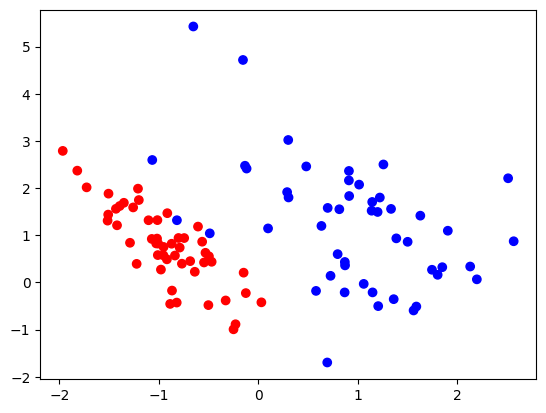
And we can visualize them with matplotlib. The plot shows that this data set is nearly linearly separable. The blue class has a couple of extreme values or outliers.
# Plot the data
plt.scatter(data[:, 0], data[:, 1], c=labels, cmap=colors_bright)
<matplotlib.collections.PathCollection at 0x7fcce8c88520>
Now, we define a function that tests given classifier with our data set.
When training a supervised machine learning algorithm, we want to be able to verify that the resulting model works on new data. We need to test that the model generalizes to unseen data. Therefore, we always split the data set into training and test sets.
Then we train the classifier on the training set. This is called fitting the model.
def run_classifier(classifier, X, y):
    datasets = train_test_split(X, y, test_size=.4, random_state=42)
    X_train, X_test, y_train, y_test = datasets
    classifier.fit(X_train, y_train)
    plot_boundary(classifier, X, datasets)
Support-vector machine (SVM) classifier#
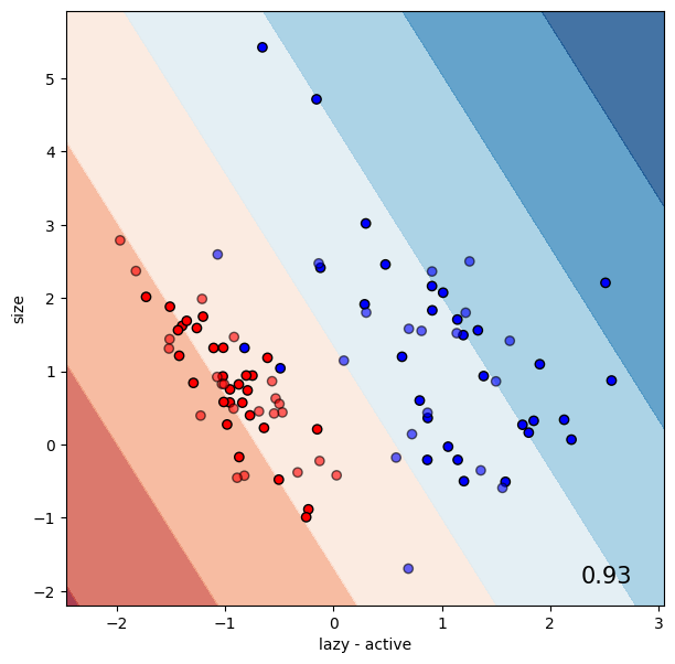
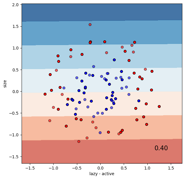
Let’s try a linear SVM classifier. The accuracy on the test set is listed in the lower right corner of the plot.
classifier = SVC(kernel="linear", C=0.025)
run_classifier(classifier, data, labels)
We can use this classifier on new data. This is also called predicting their classes or labels.
print(classifier.predict([[1.1, 2.0],
                          [-1, -2]]))
[1 0]
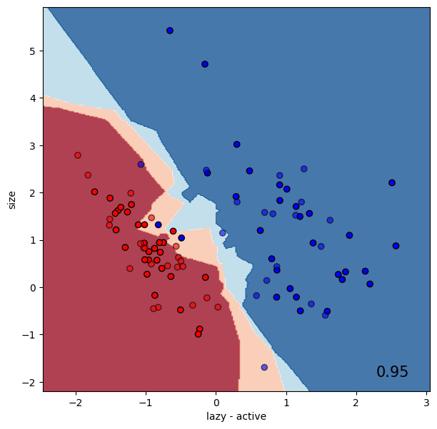
k-Nearest Neighbors (kNN)#
k-Nearest Neighbors (kNN) is an efficient classifier. kNN assigns a data point the same class as the majority of its neighbors. The value k specifies how many neighbors should be considered.
classifier = KNeighborsClassifier(3)
run_classifier(classifier, data, labels)
Linearly separable data#
The data we have worked with so far, are (nearly) linearly separable. Let’s try the SVM and kNN classifiers with a data set that is not linearly separable.
data2, labels2 = make_circles(noise=0.2, factor=0.5)
The linear SVM classifier works poorly with this data set, and yields a low accuracy.
classifier = SVC(kernel="linear", C=0.025)
run_classifier(classifier, data2, labels2)
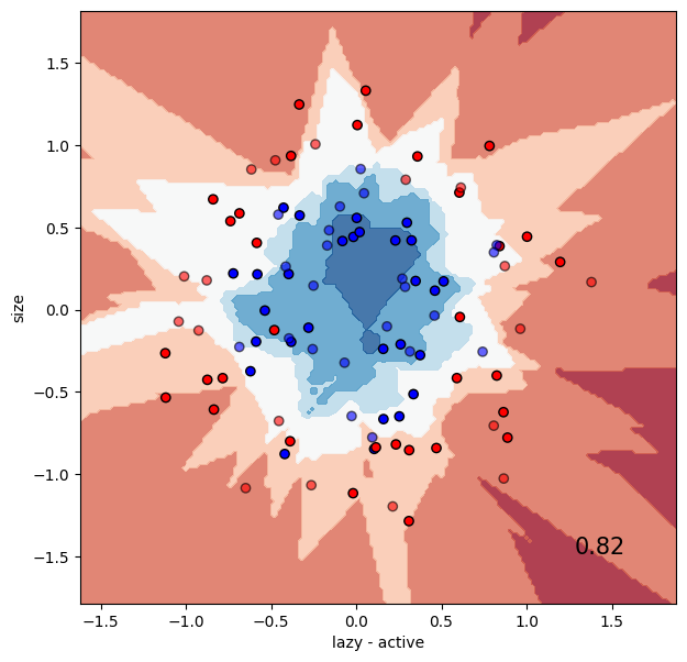
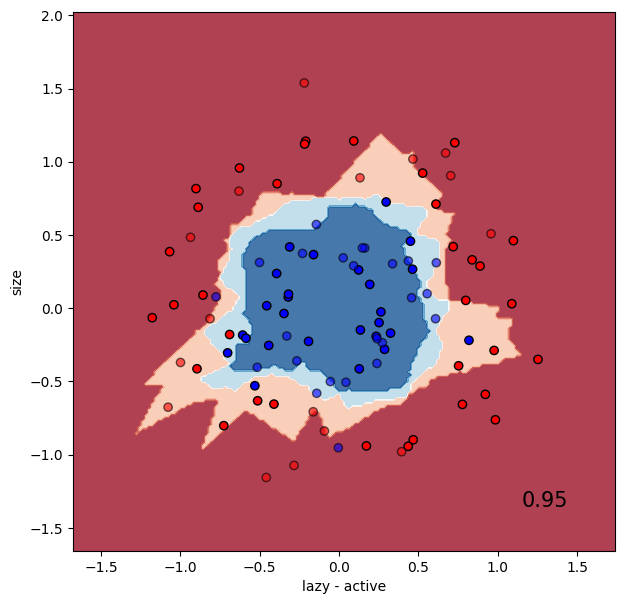
kNN, on the other hand, works well with data that is not linearly separable.
classifier = KNeighborsClassifier(3)
run_classifier(classifier, data2, labels2)
Unsupervised clustering#
In unsupervised learning there are no labels. The task is to find patterns in the data, for example by clustering them. We avoid the human effort to label the data but get less information as a result.
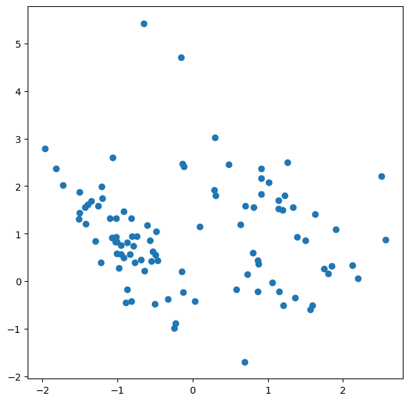
First, let’s plot the unlabeled data.
figure = plt.figure(figsize=(7, 7))
plt.scatter(data[:, 0], data[:, 1])#, s=5, linewidth=0)
<matplotlib.collections.PathCollection at 0x7fcce684d270>
k-means clustering#
k-means clustering is a common clustering algorithm. It takes the parameter k, which specifies the number of clusters we want to find. In other words, the user needs to know beforehand, a priori, how many clusters they wish to look for. We can of course try different values for k, to see which works better.
Kmean = KMeans(n_clusters=2)
Kmean.fit(data)
clusters = Kmean.predict(data)
figure = plt.figure(figsize=(7, 7))
plt.scatter(data[:, 0], data[:, 1])#, s=5)#, linewidth=0, c=clusters)
for cluster_x, cluster_y in Kmean.cluster_centers_:
    plt.scatter(cluster_x, cluster_y, s=100, c='r', marker='x')

Exercises#
Exercise: Decision tree classifier#
Below, we define a decision tree classifier. Use this classifier to classify both our data sets, data and data2. Discuss and explain the results, especially the decision boundary.
from sklearn.tree import DecisionTreeClassifier

decision_tree_classifier = DecisionTreeClassifier(max_depth=5)
# your code here
Exercise: Neural network classifier#
Below, we define two neural network classifiers. Use these classifiers to classify both our data sets, data and data2. Compare and discuss the results. What does the decision boundary tell us about these classifiers?
single_layer_network = Perceptron()
multi_layer_network = MLPClassifier(max_iter=1000)

# your code here
Exercise: k-Nearest Neighbors (kNN) classifier#
This is the same kNN classifier as we saw above. Try out different values for k and the number of data points, n_samples. Can you find a good value for k for 300 samples?
The accuracy score is in the lower right corner of the plot. Which accuracy do you get?
data3, labels3 = make_circles(n_samples = 100, noise=0.2, factor=0.5, random_state=5)

kNN_classifier = KNeighborsClassifier(10)
run_classifier(kNN_classifier, data3, labels3)